Chapter 14: Mathematical Foundations
Contents
Software professionals live with programs. In a very simple language, one can program only for something that follows a well-understood, nonambiguous logic. The Mathematical Foundations knowledge area (KA) helps software engineers comprehend this logic, which in turn is translated into programming language code. The mathematics that is the primary focus in this KA is quite different from typical arithmetic, where numbers are dealt with and discussed. Logic and reasoning are the essence of mathematics that a software engineer must address.
Mathematics, in a sense, is the study of formal systems. The word “formal” is associated with preciseness, so there cannot be any ambiguous or erroneous interpretation of the fact. Mathematics is therefore the study of any and all certain truths about any concept. This concept can be about numbers as well as about symbols, images, sounds, video—almost anything. In short, not only numbers and numeric equations are subject to preciseness. On the contrary, a software engineer needs to have a precise abstraction on a diverse application domain.
The SWEBOK Guide’s Mathematical Foundations KA covers basic techniques to identify a set of rules for reasoning in the context of the system under study. Anything that one can deduce following these rules is an absolute certainty within the context of that system. In this KA, techniques that can represent and take forward the reasoning and judgment of a software engineer in a precise (and therefore mathematical) manner are defined and discussed. The language and methods of logic that are discussed here allow us to describe mathematical proofs to infer conclusively the absolute truth of certain concepts beyond the numbers. In short, you can write a program for a problem only if it follows some logic. The objective of this KA is to help you develop the skill to identify and describe such logic. The emphasis is on helping you understand the basic concepts rather than on challenging your arithmetic abilities.
The breakdown of topics for the Mathematical Foundations KA is shown in Figure 14.1.
1 Set, Relations, Functions
Set. A set is a collection of objects, called elements of the set. A set can be represented by listing its elements between braces, e.g., S = {1, 2, 3}.
The symbol ∈ is used to express that an element belongs to a set, or—in other words—is a member of the set. Its negation is represented by ∉, e.g., 1 ∈ S, but 4 ∉ S.
In a more compact representation of set using set builder notation, {x | P(x)} is the set of all x such that P(x) for any proposition P(x) over any universe of discourse. Examples for some important sets include the following:
- N = {0, 1, 2, 3, …} = the set of nonnegative integers.
- Z = {…, −3, −2, −1, 0, 1, 2, 3, …} = the set of integers.
Finite and Infinite Set. A set with a finite number of elements is called a finite set. Conversely, any set that does not have a finite number of elements in it is an infinite set. The set of all natural numbers, for example, is an infinite set.
Cardinality. The cardinality of a finite set S is the number of elements in S. This is represented |S|, e.g., if S = {1, 2, 3}, then |S| = 3.
Universal Set. In general S = {x ∈ U | p(x)}, where U is the universe of discourse in which the predicate P(x) must be interpreted. The “universe of discourse” for a given predicate is often referred to as the universal set. Alternately, one may define universal set as the set of all elements.
Set Equality. Two sets are equal if and only if they have the same elements, i.e.:
- X = Y ≡ ∀p (p ∈ X ↔ p ∈ Y).
Subset. X is a subset of set Y, or X is contained in Y, if all elements of X are included in Y. This is denoted by X ⊆ Y. In other words, X ⊆ Y if and only if ∀p (p ∈ X → p ∈ Y). For example, if X = {1, 2, 3} and Y = {1, 2, 3,4, 5}, then X ⊆ Y. If X is not a subset of Y, it is denoted as X ⊈ Y.
Proper Subset. X is a proper subset of Y (denoted by X ⊂ Y) if X is a subset of Y but not equal to Y, i.e., there is some element in Y that is not in X. In other words, X ⊂ Y if (X ⊆ Y) ∧ (X ≠ Y). For example, if X = {1, 2, 3}, Y = {1, 2, 3, 4}, and Z = {1, 2, 3}, then X ⊂ Y, but X is not a proper subset of Z. Sets X and Z are equal sets. If X is not a proper subset of Y, it is denoted as X ⊄ Y.
Superset. If X is a subset of Y, then Y is called a superset of X. This is denoted by Y ⊇ X, i.e., Y ⊇ X if and only if X ⊆ Y. For example, if X = {1, 2, 3} and Y = {1, 2, 3,4, 5}, then Y ⊇ X.
Empty Set. A set with no elements is called an empty set. An empty set, denoted by ∅, is also referred to as a null or void set.
Power Set. The set of all subsets of a set X is called the power set of X. It is represented as ℘(X). For example, if X = {a, b, c}, then ℘(X) = {∅,{a}, {b}, {c}, {a, b}, {a, c}, {b, c}, {a, b, c}}. If |X| = n, then |℘(X)| = 2n.
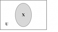
Venn Diagrams. Venn diagrams are graphic representations of sets as enclosed areas in the plane. For example, in Figure 14.2, the rectangle represents the universal set and the shaded region represents a set X.
1.1 Set Operations
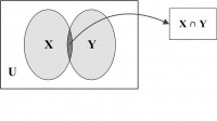
Intersection. The intersection of two sets X and Y, denoted by X ∩ Y, is the set of common elements in both X and Y. In other words, X ∩ Y = {p | (p ∈ X) ∧ (p ∈ Y)}. As, for example, {1, 2, 3} ∩ {3, 4, 6} = {3}. If X ∩ Y = f, then the two sets X and Y are said to be a disjoint pair of sets.
A Venn diagram for set intersection is shown in Figure 14.3. The common portion of the two sets represents the set intersection.
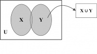
Union. The union of two sets X and Y, denoted by X ∪ Y, is the set of all elements either in X, or in Y, or in both. In other words, X ∪ Y = {p | (p ∈ X) ∨ (p ∈ Y)}. As, for example, {1, 2, 3} ∪ {3, 4, 6} = {1, 2, 3, 4, 6}. It may be noted that |X ∪ Y| = |X| + |Y| − |X ∩ Y|.
A Venn diagram illustrating the union of two sets is represented by the shaded region in Figure 14.4.
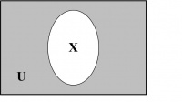
Complement. The set of elements in the universal set that do not belong to a given set X is called its complement set X'. In other words, X' ={p | (p ∈ U) ∧ (p ∉ X)}. The shaded portion of the Venn diagram in Figure 14.5 represents the complement set of X
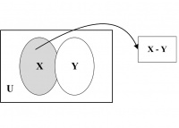
Set Difference or Relative Complement. The set of elements that belong to set X but not to set Y builds the set difference of Y from X. This is represented by X − Y. In other words, X − Y = {p | (p ∈ X) ∧ (p ∉ Y)}. As, for example, {1, 2, 3} − {3, 4, 6} = {1, 2}. It may be proved that X − Y = X ∩ Y’. Set difference X – Y is illustrated by the shaded region in Figure 14.6 using a Venn diagram.
Cartesian Product. An ordinary pair {p, q} is a set with two elements. In a set, the order of the elements is irrelevant, so {p, q} = {q, p}. In an ordered pair (p, q), the order of occurrences of the elements is relevant. Thus, (p, q) ≠ (q, p) unless p = q. In general (p, q) = (s, t) if and only if p = s and q = t. Given two sets X and Y, their Cartesian product X × Y is the set of all ordered pairs (p, q) such that p ∈ X and q ∈ Y. In other words, X × Y = {(p, q) | (p ∈ X) ∧ (q ∈ Y)}. As for example, {a, b} × {1, 2} = {(a, 1), (a, 2), (b, 1), (b, 2)}
1.2 Properties of Set
Some of the important properties and laws of sets are mentioned below.
1. Associative Laws:
X ∪ (Y ∪ Z) = (X ∪ Y) ∪ Z
X ∩ (Y ∩ Z) = (X ∩ Y) ∩ Z
2. Commutative Laws:
X ∪ Y = Y ∪ X
X ∩ Y = Y ∩ X
3. Distributive Laws:
X ∪ (Y ∩ Z) = (X ∪ Y) ∩ (X ∪ Z)
X ∩ (Y ∪ Z) = (X ∩ Y) ∪ (X ∩ Z)
4. Identity Laws:
X ∪ ∅ = X
X ∩ U = X
5. Complement Laws:
X ∪ X' = U
X ∩ X' = ∅
6. Idempotent Laws:
X ∪ X = X
X ∩ X = X
7.Bound Laws:
X ∪ U = U
X ∩ ∅ = ∅
8. Absorption Laws:
X ∪ (X ∩ Y) = X
X ∩ (X ∪ Y) = X
9. De Morgan’s Laws:
(X ∪ Y)' = X' ∩ Y'
(X ∩ Y)' = X' ∪ Y'
1.3 Relation and Function
A relation is an association between two sets of information. For example, let’s consider a set of residents of a city and their phone numbers. The pairing of names with corresponding phone numbers is a relation. This pairing is ordered for the entire relation. In the example being considered, for each pair, either the name comes first followed by the phone number or the reverse. The set from which the first element is drawn is called the domain set and the other set is called the range set. The domain is what you start with and the range is what you end up with.
A function is a well-behaved relation. A relation R(X, Y) is well behaved if the function maps every element of the domain set X to a single element of the range set Y. Let’s consider domain set X as a set of persons and let range set Y store their phone numbers. Assuming that a person may have more than one phone number, the relation being considered is not a function. However, if we draw a relation between names of residents and their date of births with the name set as domain, then this becomes a well-behaved relation and hence a function. This means that, while all functions are relations, not all relations are functions. In case of a function given an x, one gets one and exactly one y for each ordered pair (x, y).
For example, let’s consider the following two relations.
- A: {(3, –9), (5, 8), (7, –6), (3, 9), (6, 3)}.
- B: {(5, 8), (7, 8), (3, 8), (6, 8)}.
Are these functions as well? In case of relation A, the domain is all the x-values, i.e., {3, 5, 6, 7}, and the range is all the y-values, i.e., {–9, –6, 3, 8, 9}. Relation A is not a function, as there are two different range values, –9 and 9, for the same x-value of 3. In case of relation B, the domain is same as that for A, i.e., {3, 5, 6, 7}. However, the range is a single element {8}. This qualifies as an example of a function even if all the x-values are mapped to the same y-value. Here, each x-value is distinct and hence the function is well behaved. Relation B may be represented by the equation y = 8.
The characteristic of a function may be verified using a vertical line test, which is stated below:
Given the graph of a relation, if one can draw a vertical line that crosses the graph in more than one place, then the relation is not a function.
In this example, both lines L1 and L2 cut the graph for the relation thrice. This signifies that for the same x-value, there are three different y-values for each of case. Thus, the relation is not a function
2 Basic Logic
2.1 Propositional Logic
A proposition is a statement that is either true or false, but not both. Let’s consider declarative sentences for which it is meaningful to assign either of the two status values: true or false. Some examples of propositions are given below.
- 1. The sun is a star
- 2. Elephants are mammals.
- 3. 2 + 3 = 5.
However, a + 3 = b is not a proposition, as it is neither true nor false. It depends on the values of the variables a and b.
The Law of Excluded Middle: For every proposition p, either p is true or p is false.
The Law of Contradiction: For every proposition p, it is not the case that p is both true and false.
Propositional logic is the area of logic that deals with propositions. A truth table displays the relationships between the truth values of propositions.
A Boolean variable is one whose value is either true or false. Computer bit operations correspond to logical operations of Boolean variables.
The basic logical operators including negation (¬ p), conjunction (p ∧ q), disjunction (p ∨ q), exclusive or (p ⊕ q), and implication (p → q) are to be studied. Compound propositions may be formed using various logical operators.
A compound proposition that is always true is a tautology. A compound proposition that is always false is a contradiction. A compound proposition that is neither a tautology nor a contradiction is a contingency.
Compound propositions that always have the same truth value are called logically equivalent (denoted by ≡). Some of the common equivalences are:
Identity laws:
p ∧ T ≡ p
p ∨ F ≡ p
Domination laws:
p ∨ T ≡ T
p ∧ F ≡ F
Idempotent laws:
p ∨ p ≡ p
p ∧ p ≡ p
Double negation law:
¬ (¬ p) ≡ p
Commutative laws:
p ∨ q ≡ q ∨ p
p ∧ q ≡ q ∧ p
Associative laws:
(p ∨ q) ∨ r ≡ p ∨ (q ∨ r)
(p ∧ q) ∧ r ≡ p ∧ (q ∧ r)
Distributive laws:
p ∨ (q ∧ r) ≡ (p ∨ q) ∧ (p ∨ r)
p ∧ (q ∨ r) ≡ (p ∧ q) ∨ (p ∧ r)
De Morgan’s laws:
¬ (p ∧ q) ≡ ¬ p ∨ ¬ q
¬ (p ∨ q) ≡ ¬ p ∧ ¬ q
2.2 Predicate Logic
A predicate is a verb phrase template that describes a property of objects or a relationship among objects represented by the variables. For example, in the sentence, The flower is red, the template is red is a predicate. It describes the property of a flower. The same predicate may be used in other sentences too.
Predicates are often given a name, e.g., “Red” or simply “R” can be used to represent the predicate is red. Assuming R as the name for the predicate is red, sentences that assert an object is of the color red can be represented as R(x), where x represents an arbitrary object. R(x) reads as x is red
Quantifiers allow statements about entire collections of objects rather than having to enumerate the objects by name.
The Universal quantifier ∀x asserts that a sentence is true for all values of variable x. For example, ∀x Tiger(x) → Mammal(x) means all tigers are mammals.
The Existential quantifier ∃x asserts that a sentence is true for at least one value of variable x. For example, ∃x Tiger(x) → Man-eater(x) means there exists at least one tiger that is a man-eater.
Thus, while universal quantification uses implication, the existential quantification naturally uses conjunction.
A variable x that is introduced into a logical expression by a quantifier is bound to the closest enclosing quantifier. A variable is said to be a free variable if it is not bound to a quantifier.
Similarly, in a block-structured programming language, a variable in a logical expression refers to the closest quantifier within whose scope it appears.
For example, in ∃x (Cat(x) ∧ ∀x (Black(x))), x in Black(x) is universally quantified. The expression implies that cats exist and everything is black.
Propositional logic falls short in representing many assertions that are used in computer science and mathematics. It also fails to compare equivalence and some other types of relationship between propositions.
For example, the assertion a is greater than 1 is not a proposition because one cannot infer whether it is true or false without knowing the value of a. Thus, propositional logic cannot deal with such sentences. However, such assertions appear quite often in mathematics and we want to infer on those assertions. Also, the pattern involved in the following two logical equivalences cannot be captured by propositional logic: “Not all men are smokers” and “Some men don’t smoke.” Each of these two propositions is treated independently in propositional logic. There is no mechanism in propositional logic to find out whether or not the two are equivalent to one another. Hence, in propositional logic, each equivalent proposition is treated individually rather than dealing with a general formula that covers all equivalences collectively.
Predicate logic is supposed to be a more powerful logic that addresses these issues. In a sense, predicate logic (also known as first-order logic or predicate calculus) is an extension of propositional logic to formulas involving terms and predicates.
3 Proof Techniques
A proof is an argument that rigorously establishes the truth of a statement. Proofs can themselves be represented formally as discrete structures.
Statements used in a proof include axioms and postulates that are essentially the underlying assumptions about mathematical structures, the hypotheses of the theorem to be proved, and previously proved theorems.
A theorem is a statement that can be shown to be true.
A lemma is a simple theorem used in the proof of other theorems.
A corollary is a proposition that can be established directly from a theorem that has been proved.
A conjecture is a statement whose truth value is unknown.
When a conjecture’s proof is found, the conjecture becomes a theorem. Many times conjectures are shown to be false and, hence, are not theorems.
3.1 Methods of Proving Theorems
Direct Proof. Direct proof is a technique to establish that the implication p → q is true by showing that q must be true when p is true.
For example, to show that if n is odd then n2−1 is even, suppose n is odd, i.e., n = 2k + 1 for some integer k: ∴ n2 = (2k + 1)2 = 4k2 + 4k + 1
As the first two terms of the Right Hand Side (RHS) are even numbers irrespective of the value of k, the Left Hand Side (LHS) (i.e., n2) is an odd number. Therefore, n2−1 is even.
Proof by Contradiction. A proposition p is true by contradiction if proved based on the truth of the implication ¬ p → q where q is a contradiction.
For example, to show that the sum of 2x + 1 and 2y − 1 is even, assume that the sum of 2x + 1 and 2y − 1is odd. In other words, 2(x + y), which is a multiple of 2, is odd. This is a contradiction. Hence, the sum of 2x + 1 and 2y − 1 is even.
An inference rule is a pattern establishing that if a set of premises are all true, then it can be deduced that a certain conclusion statement is true. The reference rules of addition, simplification, and conjunction need to be studied.
Proof by Induction. Proof by induction is done in two phases. First, the proposition is established to be true for a base case—typically for the positive integer 1. In the second phase, it is established that if the proposition holds for an arbitrary positive integer k, then it must also hold for the next greater integer, k + 1. In other words, proof by induction is based on the rule of inference that tells us that the truth of an infinite sequence of propositions P(n), ∀n ∈ [1 … ∞] is established if P(1) is true, and secondly, ∀k ∈ [2 ... n] if P(k) → P(k + 1).
It may be noted here that, for a proof by mathematical induction, it is not assumed that P(k) is true for all positive integers k. Proving a theorem or proposition only requires us to establish that if it is assumed P(k) is true for any arbitrary positive integer k, then P(k + 1) is also true. The correctness of mathematical induction as a valid proof technique is beyond discussion of the current text. Let us prove the following proposition using induction.
Proposition: The sum of the first n positive odd integers P(n) is n2.
Basis Step: The proposition is true for n = 1 as P(1) = 12 = 1. The basis step is complete.
Inductive Step: The induction hypothesis (IH) is that the proposition is true for n = k, k being an arbitrary positive integer k.
∴ 1 + 3 + 5+ … + (2k − 1) = k2
Now, it’s to be shown that P(k) → P(k + 1).
P(k + 1) = 1 + 3 + 5+ … +(2k − 1) + (2k + 1) = P(k) + (2k + 1) = k2 + (2k + 1) [using IH] = k2 + 2k + 1 = (k + 1)2
Thus, it is shown that if the proposition is true for n = k, then it is also true for n = k + 1.
The basis step together with the inductive step of the proof show that P(1) is true and the conditional statement P(k) → P(k + 1) is true for all positive integers k. Hence, the proposition is proved.
4 Basics of Counting
The sum rule states that if a task t1 can be done in n1 ways and a second task t2 can be done in n2 ways, and if these tasks cannot be done at the same time, then there are n1+ n2 ways to do either task.
- If A and B are disjoint sets, then |A ∪ B|=|A| + |B|.
- In general if A1, A2, …. , An are disjoint sets, then |A1 ∪ A2 ∪ … ∪ An| = |A1| + |A2| + … + |An|.
For example, if there are 200 athletes doing sprint events and 30 athletes who participate in the long jump event, then how many ways are there to pick one athlete who is either a sprinter or a long jumper? Using the sum rule, the answer would be 200 + 30 = 230.
The product rule states that if a task t1 can be done in n1 ways and a second task t2 can be done in n2 ways after the first task has been done, then there are n1 * n2 ways to do the procedure.
- If A and B are disjoint sets, then |A × B| = |A| * |B|.
- In general if A1, A2, …, An are disjoint sets, then |A1 × A2 × … × An| = |A1| * |A2| * …. * |An|.
For example, if there are 200 athletes doing sprint events and 30 athletes who participate in the long jump event, then how many ways are there to pick two athletes so that one is a sprinter and the other is a long jumper? Using the product rule, the answer would be 200 * 30 = 6000.
The principle of inclusion-exclusion states that if a task t1 can be done in n1 ways and a second task t2 can be done in n2 ways at the same time with t1, then to find the total number of ways the two tasks can be done, subtract the number of ways to do both tasks from n1 + n2.
- If A and B are not disjoint, |A ∪ B| = |A| + |B| − |A ∩ B|.
In other words, the principle of inclusionexclusion aims to ensure that the objects in the intersection of two sets are not counted more than once.
Recursion is the general term for the practice of defining an object in terms of itself. There are recursive algorithms, recursively defined functions, relations, sets, etc.
A recursive function is a function that calls itself. For example, we define f(n) = 3 * f(n − 1) for all n ∈ N and n ≠ 0 and f(0) = 5.
An algorithm is recursive if it solves a problem by reducing it to an instance of the same problem with a smaller input.
A phenomenon is said to be random if individual outcomes are uncertain but the long-term pattern of many individual outcomes is predictable.
The probability of any outcome for a random phenomenon is the proportion of times the outcome would occur in a very long series of repetitions.
The probability P(A) of any event A satisfies 0 ≤ P(A) ≤ 1. Any probability is a number between 0 and 1. If S is the sample space in a probability model, the P(S) = 1. All possible outcomes together must have probability of 1.
Two events A and B are disjoint if they have no outcomes in common and so can never occur together. If A and B are two disjoint events, P(A or B) = P(A) + P(B). This is known as the addition rule for disjoint events.
If two events have no outcomes in common, the probability that one or the other occurs is the sum of their individual probabilities.
Permutation is an arrangement of objects in which the order matters without repetition. One can choose r objects in a particular order from a total of n objects by using nPr ways, where, npr = n! / (n − r)!. Various notations like nPr and P(n, r) are used to represent the number of permutations of a set of n objects taken r at a time.
Combination is a selection of objects in which the order does not matter without repetition. This is different from a permutation because the order does not matter. If the order is only changed (and not the members) then no new combination is formed. One can choose r objects in any order from a total of n objects by using nCr ways, where, nCr = n! / [r! * (n − r)!].
5 Graphs and Trees
5.1 Graphs
A graph G = (V, E) where V is the set of vertices (nodes) and E is the set of edges. Edges are also referred to as arcs or links.
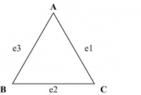
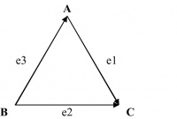
F is a function that maps the set of edges E to a set of ordered or unordered pairs of elements V. For example, in Figure 14.8, G = (V, E) where V = {A, B, C}, E = {e1, e2, e3}, and F = {(e1, (A,C)), (e2, (C, B)), (e3, (B, A))}.
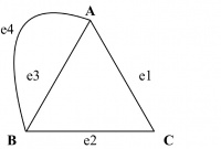
The graph in Figure 14.8 is a simple graph that consists of a set of vertices or nodes and a set of edges connecting unordered pairs. The edges in simple graphs are undirected. Such graphs are also referred to as undirected graphs. For example, in Figure 14.8, (e1, (A, C)) may be replaced by (e1, (C, A)) as the pair between vertices A and C is unordered. This holds good for the other two edges too. In a multigraph, more than one edge may connect the same two vertices. Two or more connecting edges between the same pair of vertices may reflect multiple associations between the same two vertices. Such edges are called parallel or multiple edges.
For example, in Figure 14.9, the edges e3 and e4 are both between A and B. Figure 14.9 is a multigraph where edges e3 and e4 are multiple edges.
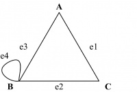
In a pseudograph, edges connecting a node to itself are allowed. Such edges are called loops.
For example, in Figure 14.10, the edge e4 both starts and ends at B. Figure 14.10 is a pseudograph in which e4 is a loop.
A directed graph G = (V, E) consists of a set of vertices V and a set of edges E that are ordered pairs of elements of V. A directed graph may contain loops.
For example, in Figure 14.11, G = (V, E) where V = {A, B, C}, E = {e1, e2, e3}, and F = {(e1, (A,C)), (e2, (B, C)), (e3, (B, A))}.
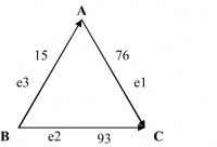
In a weighted graph G = (V, E), each edge has a weight associated with it. The weight of an edge typically represents the numeric value associated with the relationship between the corresponding two vertices.
For example, in Figure 14.12, the weights for the edges e1, e2, and e3 are taken to be 76, 93, and 15 respectively. If the vertices A, B, and C represent three cities in a state, the weights, for example, could be the distances in miles between these cities.
Let G = (V, E) be an undirected graph with edge set E. Then, for an edge e ∈ E where e = {u,v}, the following terminologies are often used:
- u, v are said to be adjacent or neighbors or connected.
- edge e is incident with vertices u and v.
- edge e connects u and v.
- vertices u and v are endpoints for edge e.
If vertex v ∈ V, the set of vertices in the undirected graph G(V, E), then:
- the degree of v, deg(v), is its number of incident edges, except that any self-loops are counted twice.
- a vertex with degree 0 is called an isolated vertex.
- a vertex of degree 1 is called a pendant vertex.
Let G(V, E) be a directed graph. If e(u, v) is an edge of G, then the following terminologies are often used:
- u is adjacent to v, and v is adjacent from u.
- e comes from u and goes to v.
- e connects u to v, or e goes from u to v.
- the initial vertex of e is u
- the terminal vertex of e is v.
If vertex v is in the set of vertices for the directed graph G(V, E), then
- in-degree of v, deg−(v), is the number of edges going to v, i.e., for which v is the terminal vertex.
- out-degree of v, deg+(v), is the number of edges coming from v, i.e., for which v is the initial vertex.
- degree of v, deg(v) = deg−(v) + deg+(v), is the sum of vs in-degree and out-degree.
- a loop at a vertex contributes 1 to both in-degree and out-degree of this vertex.
It may be noted that, following the definitions above, the degree of a node is unchanged whether we consider its edges to be directed or undirected.
In an undirected graph, a path of length n from u to v is a sequence of n adjacent edges from vertex u to vertex v.
- A path is a circuit if u=v.
- A path traverses the vertices along it.
- A path is simple if it contains no edge more than once.
A cycle on n vertices Cn for any n ≥ 3 is a simple graph where V = {v1, v2, …, vn} and E = {{v1, v2}, {v2, v3}, … , {vn−1, vn}, {vn, v1}}.
For example, Figure 14.13 illustrates two cycles of length 3 and 4.
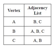
An adjacency list is a table with one row per vertex, listing its adjacent vertices. The adjacency listing for a directed graph maintains a listing of the terminal nodes for each of the vertex in the graph.
For example, Figure 14.14 illustrates the adjacency lists for the pseudograph in Figure 14.10 and the directed graph in Figure 14.11. As the out-degree of vertex C in Figure 14.11 is zero, there is no entry against C in the adjacency list.
Different representations for a graph—like adjacency matrix, incidence matrix, and adjacency lists—need to be studied.
5.2 Trees
A tree T(N, E) is a hierarchical data structure of n = |N| nodes with a specially designated root node R while the remaining n − 1 nodes form subtrees under the root node R. The number of edges |E| in a tree would always be equal to |N| − 1.
The subtree at node X is the subgraph of the tree consisting of node X and its descendants and all edges incident to those descendants. As an alternate to this recursive definition, a tree may be defined as a connected undirected graph with no simple circuits.
However, one should remember that a tree is strictly hierarchical in nature as compared to a graph, which is flat. In case of a tree, an ordered pair is built between two nodes as parent and child. Each child node in a tree is associated with only one parent node, whereas this restriction becomes meaningless for a graph where no parent-child association exists.
An undirected graph is a tree if and only if there is a unique simple path between any two of its vertices.
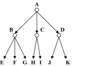
Figure 14.15 presents a tree T(N, E) where the set of nodes N = {A, B, C, D, E, F, G, H, I, J, K}. The edge set E is {(A, B), (A, C), (A, D), (B, E), (B, F), (B, G), (C, H), (C, I), (D, J), (D, K)}.
The parent of a nonroot node v is the unique node u with a directed edge from u to v. Each node in the tree has a unique parent node except the root of the tree.
For example, in Figure 14.15, root node A is the parent node for nodes B, C, and D. Similarly, B is the parent of E, F, G, and so on. The root node A does not have any parent.
A node that has children is called an internal node. For example, in Figure 14.15, node A or node B are examples of internal nodes. The degree of a node in a tree is the same as its number of children. For example, in Figure 14.15, root node A and its child B are both of degree 3. Nodes C and D have degree 2.
The distance of a node from the root node in terms of number of hops is called its level. Nodes in a tree are at different levels. The root node is at level 0. Alternately, the level of a node X is the length of the unique path from the root of the tree to node X.
For example, root node A is at level 0 in Figure 14.15. Nodes B, C, and D are at level 1. The remaining nodes in Figure 14.15 are all at level 2. The height of a tree is the maximum of the levels of nodes in the tree. For example, in Figure 14.15, the height of the tree is 2.
A node is called a leaf if it has no children. The degree of a leaf node is 0. For example, in Figure 14.15, nodes E through K are all leaf nodes with degree 0. The ancestors or predecessors of a nonroot node X are all the nodes in the path from root to node X. For example, in Figure 14.15, nodes A and D form the set of ancestors for J.
The successors or descendents of a node X are all the nodes that have X as its ancestor. For a tree with n nodes, all the remaining n − 1 nodes are successors of the root node. For example, in Figure 14.15, node B has successors in E, F, and G. If node X is an ancestor of node Y, then node Y is a successor of X.
Two or more nodes sharing the same parent node are called sibling nodes. For example, in Figure 14.15, nodes E and G are siblings. However, nodes E and J, though from the same level, are not sibling nodes. Two sibling nodes are of the same level, but two nodes in the same level are not necessarily siblings.
A tree is called an ordered tree if the relative position of occurrences of children nodes is significant. For example, a family tree is an ordered tree if, as a rule, the name of an elder sibling appears always before (i.e., on the left of) the younger sibling.
In an unordered tree, the relative position of occurrences between the siblings does not bear any significance and may be altered arbitrarily.
A binary tree is formed with zero or more nodes where there is a root node R and all the remaining nodes form a pair of ordered subtrees under the root node.
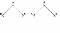
In a binary tree, no internal node can have more than two children. However, one must consider that besides this criterion in terms of the degree of internal nodes, a binary tree is always ordered. If the positions of the left and right subtrees for any node in the tree are swapped, then a new tree is derived. For example, in Figure 14.16, the two binary trees are different as the positions of occurrences of the children of A are different in the two trees.
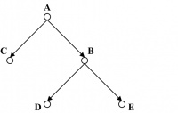
According to [1*], a binary tree is called a full binary tree if every internal node has exactly two children. For example, the binary tree in Figure 14.17 is a full binary tree, as both of the two internal nodes A and B are of degree 2. A full binary tree following the definition above is also referred to as a strictly binary tree.
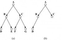
For example, both binary trees in Figure 14.18 are complete binary trees. The tree in Figure 14.18(a) is a complete as well as a full binary tree. A complete binary tree has all its levels, except possibly the last one, filled up to capacity. In case the last level of a complete binary tree is not full, nodes occur from the leftmost positions available.
Interestingly, following the definitions above, the tree in Figure 14.18(b) is a complete but not full binary tree as node B has only one child in D. On the contrary, the tree in Figure 14.17 is a full —but not complete—binary tree, as the children of B occur in the tree while the children of C do not appear in the last level. A binary tree of height H is balanced if all its leaf nodes occur at levels H or H − 1. For example, all three binary trees in Figures 14.17 and 14.18 are balanced binary trees.
There are at most 2H leaves in a binary tree of height H. In other words, if a binary tree with L leaves is full and balanced, then its height is H = ⌈log2L⌉.
For example, this statement is true for the two trees in Figures 14.17 and 14.18(a) as both trees are full and balanced. However, the expression above does not match for the tree in Figure 14.18(b) as it is not a full binary tree.
A binary search tree (BST) is a special kind of binary tree in which each node contains a distinct key value, and the key value of each node in the tree is less than every key value in its right subtree and greater than every key value in its left subtree.
A traversal algorithm is a procedure for systematically visiting every node of a binary tree. Tree traversals may be defined recursively.
If T is binary tree with root R and the remaining nodes form an ordered pair of nonnull left subtree TL and nonnull right subtree TR below R, then the preorder traversal function PreOrder(T) is defined as:
PreOrder(T) = R, PreOrder(TL), PreOrder(TR) … eqn. 1
The recursive process of finding the preorder traversal of the subtrees continues till the subtrees are found to be Null. Here, commas have been used as delimiters for the sake of improved readability.
The postorder and in-order may be similarly defined using eqn. 2 and eqn. 3 respectively.
PostOrder(T) = PostOrder(TL), PostOrder(TR), R … eqn 2
InOrder(T) = InOrder(TL), R, InOrder(TR) …eqn 3
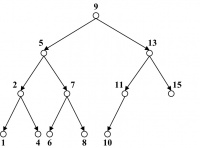
For example, the tree in Figure 14.19 is a binary search tree (BST). The preorder, postorder, and in-order traversal outputs for the BST are given below in their respective order.
Preorder output: 9, 5, 2, 1, 4, 7, 6, 8, 13, 11, 10, 15
Postorder output: 1, 4, 2, 6, 8, 7, 5, 10, 11, 15, 13, 9
In-order output: 1, 2, 4, 5, 6, 7, 8, 9, 10, 11, 13, 15
Further discussion on trees and their usage has been included in section 6, Data Structure and Representation, of the Computing Foundations KA.
6 Discrete Probability
Probability is the mathematical description of randomness. Basic definition of probability and randomness has been defined in section 4 of this KA. Here, let us start with the concepts behind probability distribution and discrete probability.
A probability model is a mathematical description of a random phenomenon consisting of two parts: a sample space S and a way of assigning probabilities to events. The sample space defines the set of all possible outcomes, whereas an event is a subset of a sample space representing a possible outcome or a set of outcomes.
A random variable is a function or rule that assigns a number to each outcome. Basically, it is just a symbol that represents the outcome of an experiment.
For example, let X be the number of heads when the experiment is flipping a coin n times. Similarly, let S be the speed of a car as registered on a radar detector.
The values for a random variable could be discrete or continuous depending on the experiment. A discrete random variable can hold all possible outcomes without missing any, although it might take an infinite amount of time. A continuous random variable is used to measure an uncountable number of values even if an infinite amount of time is given.
For example, if a random variable X represents an outcome that is a real number between 1 and 100, then X may have an infinite number of values. One can never list all possible outcomes for X even if an infinite amount of time is allowed. Here, X is a continuous random variable. On the contrary, for the same interval of 1 to 100, another random variable Y can be used to list all the integer values in the range. Here, Y is a discrete random variable.
An upper-case letter, say X, will represent the name of the random variable. Its lower-case counterpart, x, will represent the value of the random variable.
The probability that the random variable X will equal x is:
P(X = x) or, more simply, P(x).
A probability distribution (density) function is a table, formula, or graph that describes the values of a random variable and the probability associated with these values.
Probabilities associated with discrete random variables have the following properties:
i. 0 ≤ P(x) ≤ 1 for all x
ii. ΣP(x) = 1
A discrete probability distribution can be represented as a discrete random variable.
The mean μ of a probability distribution model is the sum of the product terms for individual events and its outcome probability. In other words, for the possible outcomes x1, x2, … , xn in a sample space S if pk is the probability of outcome xk, the mean of this probability would be μ = x1p1 + x2p2 + … + xnpn.
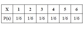
For example, the mean of the probability density for the distribution in Figure 14.20 would be
1 * (1/6) + 2 * (1/6) + 3 * (1/6) + 4 * (1/6) + 5 * (1/6) + 6 * (1/6) = 21 * (1/6) = 3.5
Here, the sample space refers to the set of all possible outcomes.
The variance s2 of a discrete probability model is: s2 = (x1 – μ)2p1 + (x2 – μ)2p2 + … + (xk – μ)2pk.
The standard deviations is the square root of the variance.
For example, for the probability distribution in Figure 14.20, the variation σ2 would be
s2 = [(1 – 3.5)2 * (1/6) + (2 – 3.5)2 * (1/6) + (3 – 3.5)2 * (1/6) + (4 – 3.5)2 * (1/6) + (5 – 3.5)2 * (1/6) + (6 – 3.5)2 * (1/6)] = (6.25 + 2.25 + 0.25 + 0.5 + 2.25 + 6.25) * (1/6) = 17.5 * (1/6) = 2.90
∴ standard deviation s =
These numbers indeed aim to derive the average value from repeated experiments. This is based on the single most important phenomenon of probability, i.e., the average value from repeated experiments is likely to be close to the expected value of one experiment. Moreover, the average value is more likely to be closer to the expected value of any one experiment as the number of experiments increases.
7 Finite State Machines
A computer system may be abstracted as a mapping from state to state driven by inputs. In other words, a system may be considered as a transition function T: S × I → S × O, where S is the set of states and I, O are the input and output functions. If the state set S is finite (not infinite), the system is called a finite state machine (FSM).
Alternately, a finite state machine (FSM) is a mathematical abstraction composed of a finite number of states and transitions between those states. If the domain S × I is reasonably small, then one can specify T explicitly using diagrams similar to a flow graph to illustrate the way logic flows for different inputs. However, this is practical only for machines that have a very small information capacity.
An FSM has a finite internal memory, an input feature that reads symbols in a sequence and one at a time, and an output feature.
The operation of an FSM begins from a start state, goes through transitions depending on input to different states, and can end in any valid state. However, only a few of all the states mark a successful flow of operation. These are called accept states.
The information capacity of an FSM is C = log |S|. Thus, if we represent a machine having an information capacity of C bits as an FSM, then its state transition graph will have |S| = 2C nodes.
A finite state machine is formally defined as M = (S, I, O, f, g, s0).
- S is the state set;
- I is the set of input symbols;
- O is the set of output symbols;
- f is the state transition function;
- g is the output function;
- and s0 is the initial state.
Given an input x ∈ I on state Sk, the FSM makes a transition to state Sh following state transition function f and produces an output y ∈ O using the output function g.
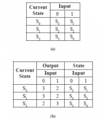
For example, Figure 14.21 illustrates an FSM with S0 as the start state and S1 as the final state. Here, S = {S0, S1, S2}; I = {0, 1}; O = {2, 3}; f(S0, 0) = S2, f(S0, 1) = S1, f(S1, 0) = S2, f(S1, 1) = S2, f(S2, 0) = S2, f(S2, 1) = S0; g(S0, 0) = 3, g(S0, 1) = 2, g(S1, 0) = 3, g(S1, 1) = 2, g(S2, 0) = 2, g(S2, 1) = 3.
The state transition and output values for different inputs on different states may be represented using a state table. The state table for the FSM in Figure 14.21 is shown in Figure 14.22. Each pair against an input symbol represents the new state and the output symbol.
For example, Figures 14.22(a) and 14.22(b) are two alternate representations of the FSM in Figure 14.21.
8 Grammars
The grammar of a natural language tells us whether a combination of words makes a valid sentence. Unlike natural languages, a formal language is specified by a well-defined set of rules for syntaxes. The valid sentences of a formal language can be described by a grammar with the help of these rules, referred to as production rules.
A formal language is a set of finite-length words or strings over some finite alphabet, and a grammar specifies the rules for formation of these words or strings. The entire set of words that are valid for a grammar constitutes the language for the grammar. Thus, the grammar G is any compact, precise mathematical definition of a language L as opposed to just a raw listing of all of the language’s legal sentences or examples of those sentences.
A grammar implies an algorithm that would generate all legal sentences of the language. There are different types of grammars.
A phrase-structure or Type-0 grammar G = (V,T, S, P) is a 4-tuple in which:
- V is the vocabulary, i.e., set of words.
- T ⊆ V is a set of words called terminals.
- S ∈ N is a special word called the start symbol.
- P is the set of productions rules for substituting one sentence fragment for another.
There exists another set N = V − T of words called nonterminals. The nonterminals represent concepts like noun. Production rules are applied on strings containing nonterminals until no more nonterminal symbols are present in the string. The start symbol S is a nonterminal.
The language generated by a formal grammar G, denoted by L(G), is the set of all strings over the set of alphabets V that can be generated, starting with the start symbol, by applying production rules until all the nonterminal symbols are replaced in the string.
For example, let G = ({S, A, a, b}, {a, b}, S, {S → aA, S → b, A → aa}). Here, the set of terminals are N = {S, A}, where S is the start symbol. The three production rules for the grammar are given as P1: S → aA; P2: S → b; P3: A → aa.
Applying the production rules in all possible ways, the following words may be generated from the start symbol.
S → aA (using P1 on start symbol)
→ aaa (using P3)
S → b (using P2 on start symbol)
Nothing else can be derived for G. Thus, the language of the grammar G consists of only two words: L(G) = {aaa, b}.
8.1 Language Recognition
Formal grammars can be classified according to the types of productions that are allowed. The Chomsky hierarchy (introduced by Noam Chomsky in 1956) describes such a classification scheme.
As illustrated in Figure 14.23, we infer the following on different types of grammars:
- 1. Every regular grammar is a context-free grammar (CFG).
- 2. Every CFG is a context-sensitive grammar (CSG).
- 3. Every CSG is a phrase-structure grammar (PSG).
Context-Sensitive Grammar: All fragments in the RHS are either longer than the corresponding fragments in the LHS or empty, i.e., if b → a, then |b| < |a| or a = ∅.
A formal language is context-sensitive if a context- sensitive grammar generates it. Context-Free Grammar: All fragments in the LHS are of length 1, i.e., if A → a, then |A| = 1 for all A ∈ N.
The term context-free derives from the fact that A can always be replaced by a, regardless of the context in which it occurs.
A formal language is context-free if a contextfree grammar generates it. Context-free languages are the theoretical basis for the syntax of most programming languages.
Regular Grammar. All fragments in the RHS are either single terminals or a pair built by a terminal and a nonterminal; i.e., if A → a, then either a ∈ T, or a = cD, or a = Dc for c ∈ T, D ∈ N.
If a = cD, then the grammar is called a right linear grammar. On the other hand, if a = Dc, then the grammar is called a left linear grammar. Both the right linear and left linear grammars are regular or Type-3 grammar.
The language L(G) generated by a regular grammar G is called a regular language.
A regular expression A is a string (or pattern) formed from the following six pieces of information: a ∈ S, the set of alphabets, e, 0 and the operations, OR (+), PRODUCT (.), CONCATENATION (*). The language of G, L(G) is equal to all those strings that match G, L(G) = {x ∈ S*|x matches G}.
For any a ∈ S, L(a) = a; L(e) = {ε}; L(0) = 0. + functions as an or, L(A + B) = L(A) ∪ L(B). . creates a product structure, L(AB) = L(A) . L(B). denotes concatenation, L(A*) = {x1x2…xn | xi ∈ L(A) and n ³ 0}
For example, the regular expression (ab)* matches the set of strings: {e, ab, abab, ababab, abababab, …}.
For example, the regular expression (aa)* matches the set of strings on one letter a that have even length.
For example, the regular expression (aaa)* + (aaaaa)* matches the set of strings of length equal to a multiple of 3 or 5.
9 Numerical Precision, Accuracy, and Errors
The main goal of numerical analysis is to develop efficient algorithms for computing precise numerical values of functions, solutions of algebraic and differential equations, optimization problems, etc.
A matter of fact is that all digital computers can only store finite numbers. In other words, there is no way that a computer can represent an infinitely large number—be it an integer, rational number, or any real or all complex numbers (see section 10, Number Theory). So the mathematics of approximation becomes very critical to handle all the numbers in the finite range that a computer can handle.
Each number in a computer is assigned a location or word, consisting of a specified number of binary digits or bits. A k bit word can store a total of N = 2k different numbers.
For example, a computer that uses 32 bit arithmetic can store a total of N = 232 ≈ 4.3 × 10⁹ different numbers, while another one that uses 64 bits can handle N’ = 264 ≈ 1.84 × 10¹⁹ different numbers. The question is how to distribute these N numbers over the real line for maximum efficiency and accuracy in practical computations.
One evident choice is to distribute them evenly, leading to fixed-point arithmetic. In this system, the first bit in a word is used to represent a sign and the remaining bits are treated for integer values. This allows representation of the integers from 1 − ½N, i.e., = 1 − 2k−1 to 1. As an approximating method, this is not good for noninteger numbers.
Another option is to space the numbers closely together—say with a uniform gap of 2−n—and so distribute the total N numbers uniformly over the interval −2−n−1N < x ≤ 2−n−1N. Real numbers lying between the gaps are represented by either rounding (meaning the closest exact representative) or chopping (meaning the exact representative immediately below —or above, if negative—the number).
Numbers lying beyond the range must be represented by the largest (or largest negative) number that can be represented. This becomes a symbol for overflow. Overflow occurs when a computation produces a value larger than the maximum value in the range.
When processing speed is a significant bottleneck, the use of the fixed-point representations is an attractive and faster alternative to the more cumbersome floating-point arithmetic most commonly used in practice.
Let’s define a couple of very important terms: accuracy and precision as associated with numerical analysis.
Accuracy is the closeness with which a measured or computed value agrees with the true value. Precision, on the other hand, is the closeness with which two or more measured or computed values for the same physical substance agree with each other. In other words, precision is the closeness with which a number represents an exact value.
Let x be a real number and let x* be an approximation. The absolute error in the approximation x* ≈ x is defined as | x* − x |. The relative error is defined as the ratio of the absolute error to the size of x, i.e., |x* − x| / | x |, which assumes x ¹ 0; otherwise, relative error is not defined.
For example, 1000000 is an approximation to 1000001 with an absolute error of 1 and a relative error of 10−6, while 10 is an approximation of 11 with an absolute error of 1 and a relative error of 0.1. Typically, relative error is more intuitive and the preferred determiner of the size of the error. The present convention is that errors are always ≥ 0, and are = 0 if and only if the approximation is exact.
An approximation x* has k significant decimal digits if its relative error is < 5 × 10−k−1. This means that the first k digits of x* following its first nonzero digit are the same as those of x.
Significant digits are the digits of a number that are known to be correct. In a measurement, one uncertain digit is included.
For example, measurement of length with a ruler of 15.5 mm with ±0.5 mm maximum allowable error has 2 significant digits, whereas a measurement of the same length using a caliper and recorded as 15.47 mm with ±0.01 mm maximum allowable error has 3 significant digits.
10 Number Theory
Number theory is one of the oldest branches of pure mathematics and one of the largest. Of course, it concerns questions about numbers, usually meaning whole numbers and fractional or rational numbers. The different types of numbers include integer, real number, natural number, complex number, rational number, etc.
10.1 Divisibility
Let’s start this section with a brief description of each of the above types of numbers, starting with the natural numbers.
Natural Numbers. This group of numbers starts at 1 and continues: 1, 2, 3, 4, 5, and so on. Zero is not in this group. There are no negative or fractional numbers in the group of natural numbers. The common mathematical symbol for the set of all natural numbers is N.
Whole Numbers. This group has all of the natural numbers in it plus the number 0.
Unfortunately, not everyone accepts the above definitions of natural and whole numbers. There seems to be no general agreement about whether to include 0 in the set of natural numbers.
Many mathematicians consider that, in Europe, the sequence of natural numbers traditionally started with 1 (0 was not even considered to be a number by the Greeks). In the 19th century, set theoreticians and other mathematicians started the convention of including 0 in the set of natural numbers.
Integers. This group has all the whole numbers in it and their negatives. The common mathematical symbol for the set of all integers is Z, i.e., Z = {…, −3, −2, −1, 0, 1, 2, 3, …}.
Rational Numbers. These are any numbers that can be expressed as a ratio of two integers. The common symbol for the set of all rational numbers is Q. Rational numbers may be classified into three types, based on how the decimals act. The decimals either do not exist, e.g., 15, or, when decimals do exist, they may terminate, as in 15.6, or they may repeat with a pattern, as in 1.666..., (which is 5/3).
Irrational Numbers. These are numbers that cannot be expressed as an integer divided by an integer. These numbers have decimals that never terminate and never repeat with a pattern, e.g., PI or √2.
Real Numbers. This group is made up of all the rational and irrational numbers. The numbers that are encountered when studying algebra are real numbers. The common mathematical symbol for the set of all real numbers is R.
Imaginary Numbers. These are all based on the imaginary number i. This imaginary number is equal to the square root of −1. Any real number multiple of i is an imaginary number, e.g., i, 5i, 3.2i, −2.6i, etc.
Complex Numbers. A complex number is a combination of a real number and an imaginary number in the form a + bi. The real part is a, and b is called the imaginary part. The common mathematical symbol for the set of all complex numbers is C.
For example, 2 + 3i, 3−5i, 7.3 + 0i, and 0 + 5i. Consider the last two examples:
7.3 + 0i is the same as the real number 7.3. Thus, all real numbers are complex numbers with zero for the imaginary part. Similarly, 0 + 5i is just the imaginary number 5i. Thus, all imaginary numbers are complex numbers with zero for the real part.
Elementary number theory involves divisibility among integers. Let a, b ∈ Z with a ≠ 0.The expression a|b, i.e., a divides b if ∃c ∈ Z: b = ac, i.e., there is an integer c such that c times a equals b.
For example, 3|−12 is true, but 3|7 is false.
If a divides b, then we say that a is a factor of b or a is a divisor of b, and b is a multiple of a. b is even if and only if 2|b.
Let a, d ∈ Z with d > 1. Then a mod d denotes that the remainder r from the division algorithm with dividend a and divisor d, i.e., the remainder when a is divided by d. We can compute (a mod d) by: a − d * ⌊a/d⌋, where ⌊a/d⌋ represents the floor of the real number.
Let Z+ = {n ∈ Z | n > 0} and a, b ∈ Z, m ∈ Z+, then a is congruent to b modulo m, written as a ≡ b (mod m), if and only if m | a−b.
10.2 Prime Number, GCD
An integer p > 1 is prime if and only if it is not the product of any two integers greater than 1, i.e., p is prime if p > 1 ∧ ∃ ¬ a, b ∈ N: a > 1, b > 1, a * b = p.
The only positive factors of a prime p are 1 and p itself. For example, the numbers 2, 13, 29, 61, etc. are prime numbers. Nonprime integers greater than 1 are called composite numbers. A composite number may be composed by multiplying two integers greater than 1.
There are many interesting applications of prime numbers; among them are the publickey cryptography scheme, which involves the exchange of public keys containing the product p*q of two random large primes p and q (a private key) that must be kept secret by a given party. The greatest common divisor gcd(a, b) of integers a, b is the greatest integer d that is a divisor both of a and of b, i.e.,
d = gcd(a, b) for max(d: d|a ∧ d|b)
For example, gcd(24, 36) = 12.
Integers a and b are called relatively prime or coprime if and only if their GCD is 1.
For example, neither 35 nor 6 are prime, but they are coprime as these two numbers have no common factors greater than 1, so their GCD is 1.
A set of integers X = {i1, i2, …} is relatively prime if all possible pairs ih, ik, h ≠ k drawn from the set X are relatively prime.
11 Algebraic Structures
This section introduces a few representations used in higher algebra. An algebraic structure consists of one or two sets closed under some operations and satisfying a number of axioms, including none.
For example, group, monoid, ring, and lattice are examples of algebraic structures. Each of these is defined in this section.
11.1 Group
A set S closed under a binary operation • forms a group if the binary operation satisfies the following four criteria:
- Associative: ∀a, b, c ∈ S, the equation (a • b) • c = a • (b • c) holds.
- Identity: There exists an identity element I ∈ S such that for all a ∈ S, I • a = a • I = a.
- Inverse: Every element a ∈ S, has an inverse a' ∈ S with respect to the binary operation, i.e., a • a' = I; for example, the set of integers Z with respect to the addition operation is a group. The identity element of the set is 0 for
the addition operation. ∀x ∈ Z, the inverse of x would be –x, which is also included in Z.
- Closure property: ∀a, b ∈ S, the result of the operation a • b ∈ S.
- A group that is commutative, i.e., a • b = b • a, is known as a commutative or Abelian group.
The set of natural numbers N (with the operation of addition) is not a group, since there is no inverse for any x > 0 in the set of natural numbers. Thus, the third rule (of inverse) for our operation is violated. However, the set of natural number has some structure.
Sets with an associative operation (the first condition above) are called semigroups; if they also have an identity element (the second condition), then they are called monoids.
Our set of natural numbers under addition is then an example of a monoid, a structure that is not quite a group because it is missing the requirement that every element have an inverse under the operation.
A monoid is a set S that is closed under a single associative binary operation • and has an identity element I ∈ S such that for all a ∈ S, I • a = a • I = a. A monoid must contain at least one element.
For example, the set of natural numbers N forms a commutative monoid under addition with identity element 0. The same set of natural numbers N also forms a monoid under multiplication with identity element 1. The set of positive integers P forms a commutative monoid under multiplication with identity element 1.
It may be noted that, unlike those in a group, elements of a monoid need not have inverses. A monoid can also be thought of as a semigroup with an identity element.
A subgroup is a group H contained within a bigger one, G, such that the identity element of G is contained in H, and whenever h1 and h2 are in H, then so are h1 • h2 and h1−1. Thus, the elements of H, equipped with the group operation on G restricted to H, indeed form a group.
Given any subset S of a group G, the subgroup generate S and their inverses. It is the smallest subgroup of G containing S.
For example, let G be the Abelian group whose elements are G' = {0, 2, 4, 6, 1, 3, 5, 7} and whose group operation is addition modulo 8. This group has a pair of nontrivial subgroups: J = {0, 4} and H = {0, 2, 4, 6}, where J is also a subgroup of H.
In group theory, a cyclic group is a group that can be generated by a single element, in the sense that the group has an element a (called the generator of the group) such that, when written multiplicatively, every element of the group is a power of a. A group G is cyclic if G = {an for any integer n}.
Since any group generated by an element in a group is a subgroup of that group, showing that the only subgroup of a group G that contains a is G itself suffices to show that G is cyclic.
For example, the group G = {0, 2, 4, 6, 1, 3, 5, 7}, with respect to addition modulo 8 operation, is cyclic. The subgroups J = {0, 4} and H = {0, 2, 4, 6} are also cyclic.
11.2 Rings
If we take an Abelian group and define a second operation on it, a new structure is found that is different from just a group. If this second operation is associative and is distributive over the first, then we have a ring.
A ring is a triple of the form (S, +, •), where (S, +) is an Abelian group, (S, •) is a semigroup, and • is distributive over +; i.e., “ a, b, c ∈ S, the equation a • (b + c) = (a • b) + (a • c) holds. Further, if • is commutative, then the ring is said to be commutative. If there is an identity element for the • operation, then the ring is said to have an identity.
For example, (Z, +, *), i.e., the set of integers Z, with the usual addition and multiplication operations, is a ring. As (Z, *) is commutative, this ring is a commutative or Abelian ring. The ring has 1 as its identity element.
Let’s note that the second operation may not have an identity element, nor do we need to find an inverse for every element with respect to this second operation. As for what distributive means, intuitively it is what we do in elementary mathematics when performing the following change: a * (b + c) = (a * b) + (a * c).
A field is a ring for which the elements of the set, excluding 0, form an Abelian group with the second operation.
A simple example of a field is the field of rational numbers (R, +, *) with the usual addition and multiplication operations. The numbers of the format a/b ∈ R, where a, b are integers and b ≠ 0. The additive inverse of such a fraction is simply −a/b, and the multiplicative inverse is b/a provided that a ≠ 0.
[1] K. Rosen, Discrete Mathematics and Its Applications, 7th ed., McGraw-Hill, 2011.
[2] E.W. Cheney and D.R. Kincaid, Numerical Mathematics and Computing, 6th ed., Brooks/Cole, 2007.
The author thankfully acknowledges the contribution of Prof. Arun Kumar Chatterjee, Ex-Head, Department of Mathematics, Manipur University, India, and Prof. Devadatta Sinha, Ex-Head, Department of Computer Science and Engineering, University of Calcutta, India, in preparing this chapter on Mathematical Foundations.

